Static Vs. Dynamic Dispersion Modeling

  Dispersion modeling defines the relationship between the emission source and the receptor. While control measures may be applied to the emission source, compliance with odor nuisance standards depend on whether the odor concentrations at the receptor have been adequately reduced with respect to their frequency, intensity, duration and location.

Luis José Marchant Santa María.¹

¹ Project Manager, Odotech Ltda, Cruz del Sur 133, oficina 503, Las Condes, Santiago, Chile, lmarchant@odotech.com

Competing interests: The author has declared that no competing interests exist.

Academic editor: Carlos N Díaz.

Content quality: This paper has not been peer reviewed due to a late arrival.

Citation: Marchant L.J., Static Vs. Dynamic Dispersion Modeling, Ist International Seminar of Odours in the Environment, 2014, Santiago, Chile, www.olores.org

Copyright: 2015 olores.org. Open Content Creative Commons license., It is allowed to download, reuse, reprint, modify, distribute, and/or copy articles in olores.org website, as long as the original authors and source are cited. No permission is required from the authors or the publishers.

Keyword: Static modeling, dynamic modeling, odor, olfactometry, electronic enose, odor master planning, odor control strategy

Download presentation

Dispersion Modeling

Dispersion modeling defines the relationship between the emission source and the receptor. While control measures may be applied to the emission source, compliance with odor nuisance standards depend on whether the odor concentrations at the receptor have been adequately reduced with respect to their frequency, intensity, duration and location.

For existing sources, it is not possible to verify compliance with nuisance odor standards by monitoring odor concentrations at the receptor because of the low odor thresholds and the variable nature of odor impacts. For new or proposed odor emission sources, dispersion modeling is also the only method to determine compliance, since the potential odor emission source does not yet exist.

Static Modeling

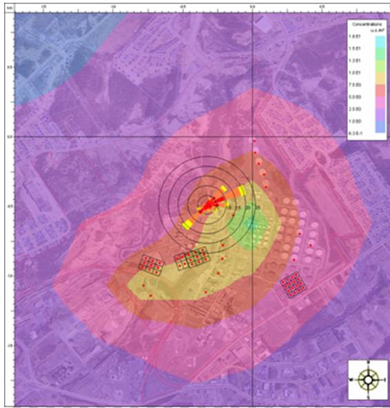
Static modeling is where the odor source is sampled during a single campaign and the olfactometric results are used to define a single steady state characterization of the source. Modeling is done using historical data (1 to 5 years). The result is a probabilistic odor impact assessment based on the pairing of "worst case" emissions with "worst case" dispersion. Compliance is based on some "acceptable" level of exceedence expressed as a percentile of number of hours. Static modeling is the only option for new or proposed odor emission sources, as the odor source does not exist and cannot be monitored. Static modeling is also called odor dispersion modeling assessment.

Figure 1: Example static modelling of the odor concentration (OU/m³) distribution centile 98.

Dynamic Modeling

Dynamic modeling is a pairing in real time of monitored odour emissions and measured meteorology. The pairing of emissions and dispersion are not independent parameters as in the case above. The critical aspect of this is that odor control measures can be applied dynamically, based on predicted exposures and not limited to controlling the worst case condition. Dynamic modelling is the preferred option where the odour emission source is large and not easily contained using conventional odour control technology.

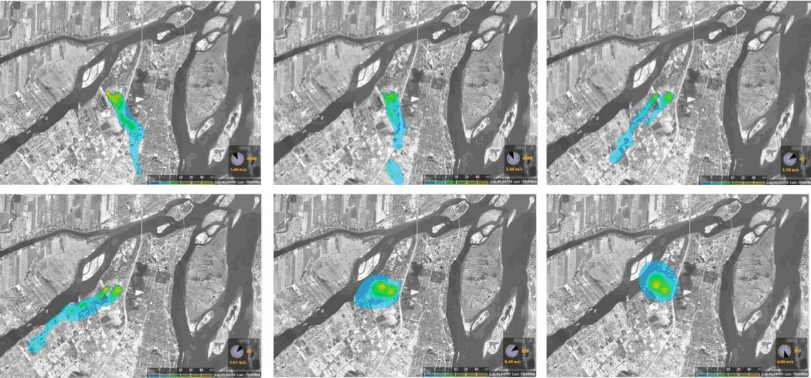
Figure 2: Example dynamic modeling of the odor concentration (OU/m3) distribution over a 24 hours period.

The current approach of olfactometry-dispersion modeling uses the odor concentrations (dilution ratios) to define the odor emission rate. The relationships between odor concentration and odor intensity, as defined by Steven's law, are not accounted for in the modeling analysis. Odor sources with the same odor concentration can have variable perceived intensities, character or hedonic tone (pleasantness or un-pleasantness). This is particularly important when odors from different sources with different odor characteristics impact a receptor simultaneously.

Odor Emissions Rates

Odor concentration as defined by olfactometry is a volume ratio and therefore dimensionless. It is given the pseudo units of “odor units per cubic meter” or OU/m³. Odor concentrations may also be described as a “dilution to threshold” ratio and be given the pseudo units of D/T. To calculate the odor emission rate for dispersion modeling analyses, the odor concentration is multiplied by the exhaust air flow rate, expressed in cubic meters per second, m³/s. The result is an odor emission rate expressed as “odor units per second” or OU/s that is compatible with dispersion modeling.

For area sources, the odor concentration is multiplied by the flux rate, expressed as “meters per second”, m/s, as determined by the type of flux chamber used to collect the sample and the surface area of the odour source. In the dispersion model, the input value may be the odor flux rate which is the product of the odor concentration and the flux rate with units of OU/m²/s.

In Static Modeling analyses, the odor emission rate would be limited to the odor concentration obtained during the sampling campaign and olfactometry analysis. The sampling procedure would be designed to characterize worst case conditions. In Dynamic Modeling analyses, the odor emission rate is directly measured continuously with electronic noses and source odor emission rates are updated live at each model iteration to account for fluctuation caused by unsteady state processes or variations causedby weather conditions.

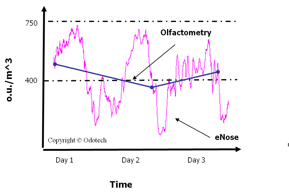
Fig. 3:Biofilter odor concentration assessment over 3 days. Snapshot olfactometry samples provide an average of 430 OU/m³ used for impact modelling. Continuous monitoring with electronic nose gives similar average but fluctuations from 150 to 700 OU/m³ fed into a dynamic modeling system.

Source Parameters

While the odor emission rate is directly proportional to the odor impact, the source characteristics at the point of release can greatly influence how effectively the odors will disperse. In modeling applications, a source may be characterized as a point, area or volume source:

• A point source is characterized as a vertical discharge through a stack or vent. It is described by the temperature and velocity of the exhaust gas, effective diameter of the open area, and release height.
• An area source is characterized as an open area where emissions are released passively through the open area, as would be the case for a quiescent basin or landfill or actively as would be the case for an aeration basin or biofilter. It is describe by the horizontal length and width of the surface area, and effective release height.
• A volume source is characterized as a horizontal release or vent that cannot be defined as either a point or area source. It may be a louver vent on the side of a building or a mobile source. It is defined as having an initial horizontal and vertical dimension, as may be described in the modeling guidance, and initial release height.

For Static Modeling analyses, the source parameters are fixed to the values that represent the worst case release scenario observed during the sampling analysis, In a Dynamic Modeling analysis, the exhaust gas temperature and exit velocity can be adjusted for each model iteration. There are fewer variables to adjust for area or volume source releases but it can consist of source location adjustments for operations that moves from day to day (landfill tipping front or composting site) or open door conditions of a sludge dewatering building or grit and screenings storage building with doors opened or closed.

Building Cavity and Wake Effects

The airflow around nearby buildings and structures can greatly influence the dispersion from point sources. Depending on the wind speed, zones of recirculating air or areas of downward moving air can increase impacts from point sources, compared to point sources not affected by a nearby structure. To account for this effect, the dimensions (length width and height) of nearby structures are entered into a modeling preprocessor algorithm along with the relative distance of the building to the point source. The output of this preprocessor is an effective building profile which potentially affects plume dispersion in each of the 36 radial directions. This building profile array is entered into the dispersion model along with the other source parameters.

While this algorithm does not apply directly to area or volume sources, the modeler may adjust the effective release height or initial dispersion dimensions of the source to account for the influence of a nearby building or structure. Buildings remain stationary and are not affected by static or dynamic modeling approaches.

Land Use Parameters

The structure of the surface boundary layer and turbulence intensity are directly related to the land use characteristics surrounding the plant site. The land use characteristics can be directly related to three parameters critical in defining turbulence intensity, surface roughness, albedo and Bowen ratio. Once the land use characteristics have been defined for a project site, they usually do not change for either the static or dynamic modeling analysis. Although, dynamic modeling could account of some changes in albedo or Bowen ratio depending on the quantity and type of precipitation:

• Surface roughness is directly proportional to the physical size of structures and vegetation. It defines the friction velocity in the surface boundary layer and the shape of the vertical wind speed profile. The surface roughness can change with the seasons if the surrounding land use is vegetated (i.e., farm land or forested). Surface roughness may also change with wind sector if an urban or suburban land use exists on one side of the plant site and field or forest exists on the other side.
• Albedo is the faction of incoming solar radiation that is reflected back to the atmosphere. The albedo is small for dark surfaces such as roads and buildings and large for bright surfaces like snow or sand. It is used to define the vertical temperature profile and the depth of the convective boundary layer.
• The Bowen ratio is related to the amount of moisture in the surface soils. Surface moisture can contribute to the release of latent heat and enhance mixing in the convective boundary layer.

Topography and Receptor Array

The receptor array contains the coordinates where plume predictions are made. The coordinates may define discrete points or a grid of points in either a polar or Cartesian reference system. The surrounding topography can greatly influence the movement of the odour plume and potential impacts on the offsite receptors. While the terrain elevations are usually accounted for in the receptor array, depending on the dispersion model being used for the analysis, topographic data may also be input to the preparation of meteorological data files.

In both static and dynamic modeling, the off-site receptor locations are where compliance with odor threshold limits is determined. In Dynamic Modeling, predicted exceedances of the odor threshold criteria can trigger measures to mitigate odor emissions before an adverse odor event occurs.

Metereological Data

Meteorological data used in a dispersion modeling analysis must be representative of weather conditions at the plant site. It defines the direction of the plume’s travel, ambient turbulence intensities and depth of the surface mixing layer. It is critical to defining the environment between the source where odors are released and receptor where compliance with odor nuisance standards is determined.

Surface Observations

In a Static Modeling analysis, historical meteorological data are taken from the nearest airport. One to five years of data may be used in a modeling study. Surface data includes, ambient temperature, wind speed, wind direction, and cloud cover. Barometric pressure, relative humidity and precipitation may also be collected, but are not used directly in modeling analysis.

The critical issue here is that the meteorological data becomes an independent variable from the odor emissions. The static modeling analysis often predicts the maximum odor impact on calm winter morning and when maximum odor emissions occur during warm summer days. Furthermore, the distance between the site and the location of the weather tower is often more than 10 to 15 km. Thus the weather data set cannot reflect the micro scale local particularities of the site and its immediate surroundings.

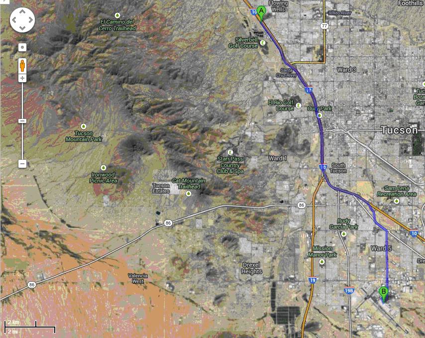
Fig 4 : Typical distance (19 km) between the source to model A (Roger Rd WWTP, Tucson) and weather station B (Tucson International Airport) available for Static dispersion modelling. Source: Google map

In a Dynamic Modeling analysis, meteorological data is collected on-site from a weather tower that is linked to the real-time monitoring system that also calculates the odor emission rate (i.e. network of eNoses at the sources). The same meteorological parameters are collected with the exception of cloud cover observations that may be replaced by solar radiation measurements. The result is the odor plume impact prediction that is overlayed on a local map and representative of the local weather conditions at that moment. As wind direction, wind speed and turbulence are by far the three most sensitive input variables for plume calculation; local measurements vastly improve the quality of the odor dispersion prediction.

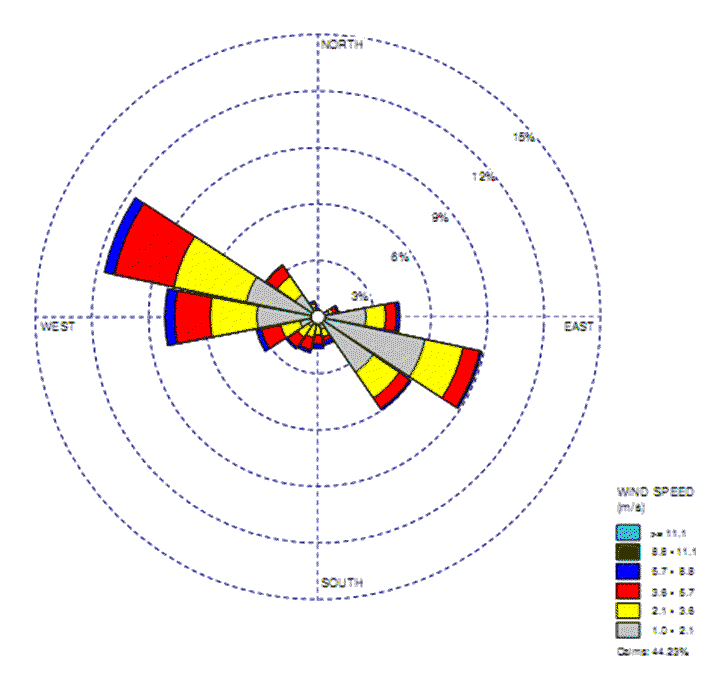
Fig 5: Roger Rd WWTP, Tucson Wind Rose for 2011 & 2013

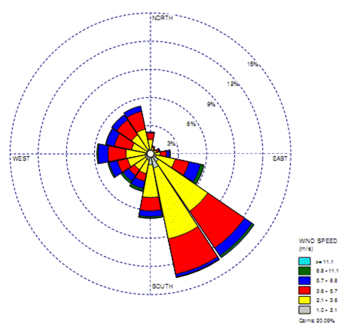
Fig 6 : Tucson Int. Airport Wind Rose for 2011 & 2013

Upper Air Data

In a Static Modeling analysis, the depth of the mixing layer is determined by radiosonde data collected by balloons that are sent upward through the depth of the atmosphere. The number of stations that perform these upper air soundings is limited and in many parts of the world the timing of the releases are not helpful in determining the depth of the mid-day convective boundary layer or the early morning stable boundary layer.

In Dynamic Modeling, measures to determine the depth of the surface mixing layer are not taken. The modeling analysis assumes an unlimited surface mixing layer. Since odor emission sources are non-buoyant, often released close to the ground and maximum predicted impacts are typically on or near the plant property boundary, this assumption does not adversely affect the results. If a hot exhaust was released from a tall stack, the lack of a cap on the surface mixing layer would be a more significant concern.

References

No references were given for this publication.